Sunday, January 31, 2010

Aqua Satellite Raw UAH Data, Part 2

In this post we take a more detailed look at the AMSU Level 1B data that serves as the raw data for UAH. Specifically, we now want to be able to write pseudocode that reads the file, checks for errors, and grabs the raw temperature data. In order to get to this level of understanding of the data, we're going to use the AIRS Version 5.0 Released Files Description PDF. It contains a section for each AIRS instrument on the Aqua satellite and each section describes every field in the Level 1B data file for that instrument.

Additional Posts In This Series
Aqua Satellite Data Processing
A Note On The UAH And RSS Raw Data
How UAH And RSS Temperatures Are Measured
Overview Of The Aqua Satellite
Looking At The Aqua Satellite Data
UAH Satellite Data
Dangit! More Climate Stuff. UAH and RSS Raw Data


Scan Information
Each AMSU Level 1B data file contains a a collection of scans that take place over 6 minutes.

In these 6 minutes, the AMSU scans 45 times in the same direction as the satellite is moving. Each of these 45 scans contains 30 readings perpendicular to the movement of the satellite (called Footprints), and each of these 30 readings contains 15 channels, each at a different height above the Earth's surface.

NOTE: These values are collected by three different pieces of hardware. Receiver A11 handles channels 6, 7, and 9 through 15. Receiver A12 handles channels 3, 4, 5, and 8. Receiver A2 handles channels 1 and 2. Also, recall from Part 1 that channel 7 is always bad. 

This gives a total of 20,250 readings in a single Level 1B file. These 20,250 readings are stored as a contiguous block of data in the file that, in the parlance of C programmers, can be read into computer memory as a three dimensional array.

There are actually two sets of this 20,250 piece block of information in the AMSU Level 1B files. The first set is called antenna temperatures and is the raw data in degrees Kelvin as read by the satellite modified by calibration information (specifically, antenna temperatures = calibration coefficient/instrument readings2).

The second set is called brightness temperatures consists of slightly modified antenna data.The brightness temperatures have a companion set of data, 20,250 error estimates called brightness temperature errors that estimate the accuracy of the brightness temperatures.

Either the antenna temperatures or the brightness temperatures can be considered to be the raw data used to create the UAH data.

Data Quality
There are several fields in the AMSU Level 1B data file that contain the results of Quality Assurance (QA) checks. In fact, much of the file is QA data. These fields tell if various pieces of data in the file can be used with confidence. Here are the important QA fields to check when processing temperature data:
  • State 1 Indicates the state of the AMSU-A1 unit for each scan line. If this value is anything other than 0, the data in the scan line should be rejected.
  • QA Receiver A11 and QA Receiver A12 These flags indicate the quality of the AMSU temperature receivers for each scan line. If either are non-zero, the data in the scan line should be rejected.
  • SATGEO QAGLINTGEO QA, and MOONGEO QA These fields contain QA information for each scan line. If a non-zero value is present, the data in the corresponding field should be rejected. 
  • FTPTGEO QA, ZENGEO QA, and DEMGEO QA These are satellite position QA flags and occur for each of the 30 field of view footprints for each of the 45 scan lines. If a non-zero value is present, the data in the corresponding field should be rejected. 
  • QA Channel This is a series of 15 flags indicating the reliability of each channel of the AMSU. Channels with non-zero values should not be used. Recall from Part 1 that channel 7 is always bad. 
Pseudocode For Reading Raw UAH Data
The following pseudocode shows how to process a AMSU Level 1B file, checking for QA errors, and grabbing the temperature data. Recall that temperatures are provided in degrees Kelvin and that channel 7 is always bad.

Open File
Read AMSU Record Into Memory

Foreach Of The 45 Scanlines
   If State_1 Not Equal To 0 Then Reject Scanline
   If QA_Receiver_A11 Not Equal To 0 Then Reject Scanline
   If QA_Receiver_A12 Not Equal To 0 Then Reject Scanline
   If SATGEO_QA Not Equal To 0 Then Reject Scanline
   If GLINTGEO_QA Not Equal To 0 Then Reject Scanline
   If MOONGEO_QA Not Equal To 0 Then Reject Scanline

   Foreach Of The 30 Footprints
      If FTPTGEO_QA Not Equal To 0 Then Reject Footprint
      If ZENGEO_QA Not Equal To 0 Then Reject Footprint
      If DEMGEO_QA Not Equal To 0 Then Reject Footprint

      Foreach Of The 15 Channels
         If QA_CHANNEL Not Equal To 0 Then Reject Channel

         Read Antenna Temperature for this Scanline/Footprint/Channel
         Read Brightness Temperature for this Scanline/Footprint/Channel
         Read Brightness Temperature Error for this Scanline/Footprint/Channel
      End Foreach
   End Foreach
End Foreach


References:
Aqua Satellite Raw UAH Data, Part 1
Aqua Satellite Data Processing
A Note On The UAH And RSS Raw Data
How UAH And RSS Temperatures Are Measured
Overview Of The Aqua Satellite
Looking At The Aqua Satellite Data
UAH Satellite Data
Dangit! More Climate Stuff. UAH and RSS Raw Data
AIRS Version 5.0 Released Files Description

Saturday, January 30, 2010

Aqua Satellite Raw UAH Data, Part 1

In this post we're going to start looking at the details of the data inside the AMSU Level 1B file that contains the raw data used to generate UAH temperatures. When downloading the data from NASA a PDF named README.AIRABRAD.pdf describing the data is included in the download and also available here. We'll be using that PDF extensively to understand the data.

Additional Posts In This Series
Satellite Summary
Aqua Satellite Data Processing
A Note On The UAH And RSS Raw Data
How UAH And RSS Temperatures Are Measured
Overview Of The Aqua Satellite
Looking At The Aqua Satellite Data
UAH Satellite Data
Dangit! More Climate Stuff. UAH and RSS Raw Data

Background
The Level 1B AMSU products contain calibrated and geolocated brightness temperatures in degrees Kelvin. The file format is currently at version 5. Version 5 first appeared in June, 2007. Highlights of the changes from Version 4 to version 5 are provided below.

• Improved Quality Indicators and Error Estimates
• Correction to Saturation and Relative Humidity
• Correction to Outgoing Longwave Radiation
• Improved O3 Product
• Addition of CO and CH4 Products
• Averaging Kernel, Verticality and Degrees of Freedom
• AMSU-A Level 1B Sidelobe Correction Implemented
• No HSB data
• Removal of VIS/NIR Derived Cloud Fields
• Preparation of AIRS-Only Processing Option

AMSU-A primarily provides temperature soundings. It is a 15-channel microwave temperature sounder implemented as two independently operated modules. Module 1 (AMSU-A1) has 12 channels in the 50-58 GHz oxygen absorption band which provide the primary temperature sounding capabilities and 1 channel at 89 GHz which provides surface and moisture information. Module 2 (AMSU-A2) has 2 channels: one at 23.8 GHz and one at 31.4 GHz which provide surface and moisture information (total precipitable water and cloud liquid water).

The AMSU-A has the three receiving antennas, two for AMSU-A1 and one for AMSU-A2, that are parabolic focusing reflectors mounted on a scan axis at a 45° Tilt angle, so that radiation is reflected from a direction along the scan axis (a 90° reflection). AMSU-A scans three times as slowly as AIRS (once per 8 seconds) and its footprints are approximately three times as large as those of AIRS (45 km at nadir). This result in three AIRS scans per AMSU-A scans and nine AIRS footprints per AMSU-A footprint.

There are 240 files that make up each days measurements. Each file is about 0.5 MB in size.

AMSU Channel 7 has a high level of noise and should not be used.

Key Data Concepts
HDF-EOS: The HDF file format is NASA's standard file format for storing data from the Earth Observing System (EOS), which is the data gathering system of sensors (mainly satellites) supporting the Global Climate Change Research Program. The Aqua satellite uses a specialized form of HDF called HDF-EOS, which deals specifically with the kinds of data that EOS produces.

Swath: The swath concept for HDF-EOS is based on a typical satellite swath, where an instrument takes a series of scans perpendicular to the ground track of the satellite as it moves along that ground track (see diagram at left). As the AIRS is profiling instrument that scans across the ground track, the data would be a three dimensional array of measurements where two of the dimensions correspond to the standard scanning dimensions (along the ground track and across the ground track), and the third dimension represents a range from the sensor. The "horizontal" dimensions can be handled as normal geographic dimensions, while the third dimensions can be handled as a special "vertical" dimension.

Major Data Groups
The AMSU Level 1B file is made of four major groups; “Dimensions”, “geolocation fields”, “Attributes”, and “Data fields” with data fields sub-divided into “Per-Granule Data Fields”, "Along-Track Data Fields, and “Full Swath Data Fields”.

Dimensions: These are HDF-EOS swath dimensions. The names "GeoTrack" and "GeoXTrack" have a special meaning for this document: "GeoTrack" is understood to be the dimension along the path of the spacecraft, and "GeoXTrack" is the dimension across the spacecraft track, starting on the left looking forward along the spacecraft track. There may also be a second across-track dimension "CalXTrack," equivalent to "GeoXTrack," except that "CalXTrack" refers to the number of calibration footprints per scanline. "GeoTrack" is 45 for large-spot products (AMSU-A, Level-2, cloud-cleared AIRS) and 135 for small-spot products (AIRS, Vis/NIR, HSB).

Geolocation Fields: These are all 64-bit floating-point fields that give the location of the data in space and time. If the note before the table specifies that these fields appear once per scanline then they have the single dimension "GeoTrack." Otherwise, they appear once per footprint per scanline and have dimensions "GeoTrack,GeoXTrack."

Attributes: These are scalar or string fields that appear only once per granule (a granule is a file). They are attributes in the HDF-EOS Swath sense.

Per-Granule Data Fields: These are fields that are valid for the entire granule (a granule is a file) but that are not scalars because they have some additional dimension.

Along-Track Data Fields: These are fields that occur once for every scanline. These fields have dimension "GeoTrack" before any "Extra Dimensions." So an "Along-Track Data Field" with "Extra Dimensions" of "None" has dimensions "GeoTrack"; whereas, if the "Extra Dimensions" is "SpaceXTrack (= 4)," then it has dimensions “GeoTrack,SpaceXTrack."

Key Data Fields
Location Data Fields
• Latitude: Boresight geodetic latitude (degrees North, -90->+90), dimension (90,135)
• Longitude: Boresight geodetic longitude (degrees East, -180->+180), dimension (90,135)
• Time: Footprint "shutter" TAI Time: floating-point elapsed seconds since Jan 1, 1993

Per-Granule Data Fields
• center_freq: Channel center frequency (GHz), dimension (15)
• IF_offset_1: Offset of first intermediate frequency stage (MHz) (zero for no mixing), dimension (15)
• IF_offset_2: Offset of second intermediate frequency stage (MHz) (zero for no second mixing), dimension (15)
• Bandwidth: Bandwidth of sum of 1,2 or 4 channels (MHz), dimension (15)
• NeDT: Instrument noise level estimated from warm count scatter (15)

Along-Track Data Fields
• qa_scanline: Bit field for each scanline (bit 0 set if sun glint in scanline; bit 1 set if costal crossing in scanline, bit 2 set if some channels had excessive NeDT estimated), dimension (45)
• qa_channel: Bit field by channel for each scanline (bit 0 set if all space view counts bad; bit 1 set if space view counts marginal; bit 2 set if space view counts could not be smoothed; bit 3 set if all blackbody counts bad; bit 4 set if blackbody counts marginal; bit 5 set if blackbody counts could not be smoothed; bit 6 set if unable to calculate calibration coefficients; bit 7 set if excessive NeDT estimated), dimension (15,45)

Swath Data Fields
• antenna_temp: Calibrated, geolocated channel-by-channel AMSU observed raw antenna temperature (K), dimension (15,30,45)
• brightness_temp: Calibrated, geolocated channel-by-channel AMSU sidelobe-corrected antenna temperature (K), dimension (15,30,45)
• brightness_temp_err: Error estimate for brightness_temp (K), dimension (15,30,45)
• landFrac: Fraction of AMSU footprint that is land (0.0 -> 1.0), dimension (30,45)
• landFrac_err: Error estimate for landFrac, dimension (30,45)

References:
Satellite Summary
Aqua Satellite Data Processing
A Note On The UAH And RSS Raw Data
How UAH And RSS Temperatures Are Measured
Overview Of The Aqua Satellite
Looking At The Aqua Satellite Data
UAH Satellite Data.html
Dangit! More Climate Stuff. UAH and RSS Raw Data
README Document for AIRS Level-1B Version 5 AMSU-A Calibrated Brightness Temperature products: AIRABRAD, AIRABRAD_NRT
AIRS/AMSU/HSB Version 5 Changes from Version 4
AIRS/AMSU/HSB Version 5 Data Disclaimer

Friday, January 29, 2010

Satellite Summary

In this post we're going to summarize the information learned so far by examining the Aqua satellite. This post lays the foundation for actually examining the data. We'll look at what we know about UAH, RSS, and the AMSR-E data.

The information here represents my current state of knowledge and supersedes information from previous posts in cases where there are differences.

Additional Posts In This Series
Aqua Satellite Data Processing
A Note On The UAH And RSS Raw Data
How UAH And RSS Temperatures Are Measured
Overview Of The Aqua Satellite
Looking At The Aqua Satellite Data
UAH Satellite Data.html
Dangit! More Climate Stuff. UAH and RSS Raw Data

UAH
UAH data is obtained from the Aqua satellite. The "Hot Load" method of calibrating the Aqua satellite failed and the satellite is now calibrated using Cosmic Background Radiation, scans from Earth and information from other satellites.

Level 0 data up to 4 days old can be obtained from the University of Wisconsin. Level 1A data is not available. Level 1B data can be obtained from the NASA AIRS data holdings web page. Level 2A data can also be obtained from the NASA AIRS data holdings web page.

RSS
RSS data is obtained from a collection of NOAA satellites. Calibration methods are unknown.

No raw data is available. Links claiming to provide raw data are dead. The final data product produced by RSS can be found here.

Due to lack of raw data, this will be the last post discussing RSS.

AMSR-E
AMSR-E data is obtained from the Aqua satellite. The "Hot Load" method of calibrating the Aqua satellite failed and the satellite is now calibrated using Cosmic Background Radiation, scans from Earth and information from other satellites.

Level 0 data up to 4 days old can be obtained from the University of Wisconsin. Level 1A data can be downloaded here. The JAXA link to the AMSR-E Level 1B data is a dead link. Level 2A data can be downloaded here.

References:
Aqua Satellite Data Processing
A Note On The UAH And RSS Raw Data
How UAH And RSS Temperatures Are Measured
Overview Of The Aqua Satellite
Looking At The Aqua Satellite Data
UAH Satellite Data.html
Dangit! More Climate Stuff. UAH and RSS Raw Data
University of Wisconsin Aqua Level 0 Data (most recent 4 days of data)
NASA AIRS data holdings web page
Dead Link For RSS Raw Data
RSS final monthly Temperature Data
EOS Data Pool @ NSIDC AMSR-E Level 1A Data.
JAXA Link To AMSR-E Level 1B Data (Dead Link).
EOS Data Pool @ NSIDC AMSR-E Level 2A Data.

Thursday, January 28, 2010

Climate Scientist Starter Kit Working With Curves


Shows how to use the Climate Scientist Starter Kit to work with curves so common to climate data.

This video has been placed in the public domain.

Wednesday, January 27, 2010

IPCC Water Vapor Statements Wrong

The IPCC is getting hit left and right these days. From the Himalayan glaciers, to Dr Rajendra Pachauri business dealings, to using non-peer reviewed Greenpeace and WWF publications over 100 times in the IPCC report, to grossly overstating the danger of warming to the rain forests, it just goes on and on.

In this post I'm going to risk a 15 yard penalty for piling on and point out that the IPCC's AR4 Technical Summary claim that the Earth's water vapor is increasing is false.

First, the claim. It comes from the IPCC's AR4 Technical Summary.
TS.3.1.3 Changes in the Water Cycle: Water Vapour, Clouds, Precipitation and Tropical Storms
Tropospheric water vapour is increasing (Figure TS.8). Surface specific humidity has generally increased since 1976 in close association with higher temperatures over both land and ocean. Total column water vapour has increased over the global oceans by 1.2 ± 0.3% per decade (95% confidence limits) from 1988 to 2004. The observed regional changes are consistent in pattern and amount with the changes in SST and the assumption of a near-constant relative humidity increase in water vapour mixing ratio. The additional atmospheric water vapour implies increased moisture availability for precipitation.

The claim is that both tropospheric and surface water vapor is increasing from 1988 to 2004. Here's a screen grab of the accompanying graph:


The top part of the graph shows the alleged increase in water vapor. The bottom part of the graph shows the increase in temperatures. The meaning is pretty clear, increased water vapor is causing the temperatures to go up.

The problem is, the amount of water vapor in the troposphere, or anywhere else, hasn't increased between 1988 to 2004 or at any time since 1983. Atmospheric water vapor is measured by NASA's ISCCP project, and the results of their measurements from June, 1983 to July, 2008 are shown in the Climate4You graph below:


Tropospheric water vapor is the middle green line and it's been holding fairly steady for the entire graph. In fact, it's actually slightly lower at the end of the graph than at the beginning, as are all the other water vapor measurements in that graph.

Once again, the IPCC is presenting bogus claims.

Water Vapor And Cosmic Rays
A relationship that does hold up is that between cosmic rays and clouds and water vapor. As cosmic rays increase or decrease, so too do clouds and water vapor. You can see the relationship between cosmic rays (brown), clouds (light blue) and water vapor (dark blue) in the graph below:

The changes in cosmic rays along with a 1 year cycle that represents the Earth revolving around the sun provide a very good correlation with changes in clouds and water vapor. The data in the graph originally comes from NASA's ISCCP and the Climax cosmic ray monitoring system. You can also get the data for the above graph from the Climate Scientist Starter Kit Spreadsheet.

References:
IPCC's Himalayan Glacier 'Mistake' No Accident
Pachauri in a spot as climategate hits TERI
More Dodgy Citations in the Nobel-Winning Climate Report
Google Search IPCC AR4 For Greenpeace
And now for Amazongate
IPCC's AR4 Technical Summary.
Climate4You
ISCCP Cloud Data
Climax Cosmic Ray Data
Climate Scientist Starter Kit Spreadsheet.

Sunday, January 24, 2010

Aqua Satellite Data Processing

In this post we look at the steps that go into processing the Aqua satellite data. We'll be looking at Level 0 (raw satellite) data to level 2A data.

Additional Posts In This Series
A Note On The UAH And RSS Raw Data
How UAH And RSS Temperatures Are Measured
Overview Of The Aqua Satellite
Looking At The Aqua Satellite Data
UAH Satellite Data.html
Dangit! More Climate Stuff. UAH and RSS Raw Data


Level 0 data is the actual data produced by the instruments on the satellite. The data has not been through Quality Assurance, it hasn't been geocoded, etc.

I'm not going to be using data at such a low level, but if you want to download it, the University of Wisconsin keeps the last four days of Level 0 data for the Aqua satellite here. Connect via FTP as an anonymous (Guest) user. See the file 00README.txt for additional information.


Level 0 AMSR-E data is processed into Level 1A data by the Japan Aerospace Exploration Agency (JAXA). Level 0 AMSU data is processed into Level 1A data by NASA. Like Level 0 data, I consider Level 1A data too low level to use.

AMSU Level 1A data contains geo-located data counts and engineering parameters. I have not been able to find AMSU Level 1A data online for downloading.

For AMSR-E Level 1A data, each half-orbit data granule consists of observation counts, antenna temperature coefficients, offsets for calculating antenna temperatures, calibration temperature counts, land/ocean flags, time, latitude, longitude, and navigation fields in HDF format. The data sampling interval is 2.6 msec for each 1.5-sec scan period for the 6.9-GHz to 36.5-GHz channels, and 1.3 msec for the 89.0-GHz channel. AMSR-E collects 243 data points per scan for the 6.9-GHz to 36.5-GHz channels, and 486 data points for the 89.0-GHz channel. Each swath spans 50 minutes.

AMSR-E Level 1A data can be downloaded here.


Level 1A AMSR-E data is processed into Level 1B data by the Japan Aerospace Exploration Agency (JAXA). Level 1A AMSU data is processed into Level 1B data by NASA.

The AMSU-A Level 1B data set contains AMSU-A calibrated and geolocated brightness temperatures in degrees Kelvin. This data set is generated from AMSU-A Level 1A digital numbers (DN) and contains 15 microwave channels in the 50 - 90 GHz and 23 - 32 GHz regions of the spectrum. A day's worth of data is divided into 240 scenes, each of 6 minute duration. An AMSU-A scene contains 30 cross-track footprints in each of 45 along-track scanlines, for a total of 45 x 30 = 1350 footprints per scene. The AMSU-A is co-aligned with the AIRS instrument onboard the Aqua platform so that successive blocks of 3 x 3 AIRS footprints are corresponding to AMSU-A footprint. The AMSU Level 1B data can be downloaded from the NASA AIRS data holdings web page. A Quick start Guide for this data is here. Code for reading Level 1B data is available for IDL, MATLAB, Fortran, and C.

AMSR-E Level 1B data is brightness temperature that is transformed from antenna temperature in level 1A by transformation coefficients. The JAXA link to the AMSR-E Level 1B data is a dead link.


Level 2A data is created from Level 1B data by either RSS or NASA. Level 2A data contains derived data and is used to produce various Level 3 and Level 4 data files.

AMSU Level 2A data contains combined data from the AIRS/AMSU/HSB instruments and can be downloaded here.

AMSR-E Level 2A data is brightness temperature that contains derived geophysical variables at the same resolution and location as the Level-1 source data. These derived data include geophysical quantities for water, water vapor, cloud liquid water, precipitation, sea surface wind speed , sea surface temperature, sea ice concentration, snow water equivalent, and soil moisture.

Recently the AMSR-E/Aqua Level 2A data was determined to have errors in the resampled 89.0 GHz Horizontal (H) fields. Files with data coverage from 19 June 2002 00:29 through 4 November 2004 05:43 are affected. The fields containing bad data are:
• 89.0H_Res.1_TB
• 89.0H_Res.2_TB
• 89.0H_Res.3_TB
• 89.0H_Res.4_TB

AMSR-E Level 2A data can be downloaded here.

An online history of of the changes made to processing this data can be found here.

References:
Guide Documents for AIRS Version 5 Products
University of Wisconsin Aqua Satellite Level 0 Data
AMSR-E/Aqua L1A Raw Observation Counts
Aqua Project Science Data Products Summary
NSIDC Data Pool
AMSR-E Format L2
JAXA/EOC (Dead Link)
NASA AIRS data holdings web page
AIRS/AMSU/HSB Version 5 Level 1B QA Quick Start
IDL AMSU Level 1B Swath and Grid Readers
MATLAB AMSU Level 1B Swath and Grid Readers
Fortran AMSU Level 1B Swath and Grid Readers
C AMSU Level 1B Swath and Grid Readers
NSIDC AMSR-E Data Frequently Asked Questions
AMSR-E Level 2 Map format description (NDX-000273D)
EOS Data Pool @ NSIDC AMSR-E Level 2A Data Download.
AMSR-E L2A Brightness Temperatures: Bad Resampled 89 GHz Horizontal Data
AMSR-E Data News

A Note On The UAH And RSS Raw Data

For those who've been following along in this series of articles, you know I've had a bit of trouble identifying exactly which files from what site contain the UAH and RSS data. This trouble continues and with this post I'll update my current thinking on situation.

UAH raw data is available from NASA at their AIRS data holdings web page as discussed in this previous post.

RSS raw data comes from NOAA, not NASA. RSS provides several links to various versions of the data. All of these links are either dead:

Monthly binary data
Read routines

or contain data that has not been updated in 3 years:

Zonally Averaged Monthly Anomalies

I'm also unable to find the data at the NOAA Comprehensive Large Array-data Stewardship System.

It's possible, of course, that I'm simply looking in the wrong place for the raw RSS data. But I was unable to find this data with reasonable effort, including following links that claimed to supply the data.

Given these difficulties in obtaining RSS raw data, I'm dropping further coverage of RSS. Coverage of the raw UAH data as well as the raw AMSR-E data will continue.

Additional Posts In This Series
How UAH And RSS Temperatures Are Measured
Overview Of The Aqua Satellite
Looking At The Aqua Satellite Data
UAH Satellite Data.html
Dangit! More Climate Stuff. UAH and RSS Raw Data

Thursday, January 21, 2010

How UAH And RSS Temperatures Are Measured

UPDATE:
On February 5th, Dr. Spencer left this not on the WUWT website: S

[NOTE: While the tropospheric temperatures we compute come from the AMSU instrument that also flies on the NASA Aqua satellite, along with the AMSR-E, there is no connection between the calibrations of these two instruments.]

So this means the AMSRU used by UAH still uses the original hot load calibration.

UPDATE:
After making this post, I discovered that RSS data comes from a NOAA satellite, but the raw data isn't available online. See this post for more information.

I'm going to continue discussing both the AMSU and the AMSR-E because there is interesting data being collected by the AMSR-E.
============

In this post we're going to take a look at how the Aqua satellite measures temperatures for UAH and RSS. We're going to be looking at some of the problems that arise in doing this, so let me start off by saying this post isn't an attack on the work done by the scientists associated with the Aqua satellite. I think UAH and RSS provide the best estimate for temperatures. Never the less, there are problems with the methodology and we're going to discuss them.

Previous posts in this series are linked below:
Overview Of The Aqua Satellite
Looking At The Aqua Satellite Data
UAH Satellite Data
Dangit! More Climate Stuff. UAH and RSS Raw Data

Public information regarding the AMSU is provided by NASA. Public information regarding the AMSR-E is provided by NSIDC. Both sources, and additional sources, were used to create this article.

Calibration
Original Calibration Process
Calibration is a process that makes instrument readings accurate and useful. Instruments are calibrated against known values so that there readings of unknown values can be considered reliable.

NOTE: The calibration process described here differs from the calibration process described by Dr. Spencer. The calibration process described here has new steps that replace the process described by Dr. Spencer. The calibration process described by Dr. Spencer is presented here, and the new process is described after the original process. I believe the new process is the correct description. I've written to Dr. Spencer in order to get his input on this.

The temperature sensing instruments on the Aqua satellite must be calibrated. The original design of the calibration had the satellite reading the temperature of the Cosmic Background Radiation (CBR) to calibrate it against a known low temperature value of 2.7 K. A high temperature calibration was done against an onboard "Hot Load" whos temperature was measured by eight precision thermostats.

With calibrated values for low and high temperatures available, values read from the Earth are simply scaled between these low and high values to determine the temperature.

However, after launch large thermal gradients due to solar heating developed within the hot load, making it difficult to determine from the thermostat readings the average effective temperature, or the temperature the radiometer sees. Because of this, a new method was needed to calibrate the satellite instruments.

New Calibration Process
The new method takes a reading from Earth and compares it against readings from other satellites measuring the same location and time. From this additional information, the Earth temperature reading for the Aqua satellite is calibrated. Then based on the temperature of the CBR and the calibrated Earth temperate, the hot load temperature is extrapolated.

Because of this, the calibration of Aqua instruments is dependent upon the calibration of these other satellites. These satellites are the TMI and SSM/I satellites. The SSM/I satellite uses the CBR and hot load calibration method that Aqua originally intended to use. The TMI satellite uses statistical analysis and calibration information from the SSM/I satellite.

The end result of this process is the instruments on the Aqua satellite are calibrated without the need for ground-based temperature measurements.

Coverage
Coverage In Space
The Aqua satellite provides coverage that is global between 89.24°N and 89.24°S. In a single day the satellite performs 28 half orbits around the Earth.

There are several small diamond-shaped areas not covered by the scans, as well as small areas of the north and south pole that are not scanned. These missing area can be seen in the accompanying diagrams presented here.


Coverage In Time


The Aqua satellite takes about 50 minutes to cover a swath of the planet. Aqua observes a given location on Earth from zero to eight times per day, depending on latitude, longitude, and phase of Aqua's orbit. This figure shows the minimum, maximum, and average number of times that Aqua observes a location at a given latitude. The average is around one-degree latitude bands.

For example, at the equator on a given day, Aqua does not observe certain longitudes that fall between orbits on that day. At other longitudes, where subsequent orbits overlap, Aqua observes that point twice per day. On the average, Aqua observes each longitude at the equator slightly more than once per day.

Scanning Process
AMSR-E Scanning Process

The AMSR-E instrument has 6 channels, or "horns" it uses to collect data from the Earth. A physical description of the horns appears in the image above and their technical specifications, including which data products (Level 1B and/or Level 2A products) their readings appear in, are described in the table below.

Link to original table
AMSR-E Spatial Characteristics of Observations
Reso-lutionFoot printMean spatial resolutionChannels
89.0 GHz36.5 GHz23.8 GHz18.7 GHz10.7 GHz6.9 GHz
1
75 km x 43 km
56 km
o
2
51 km x 29 km
38 km
o
3
27 km x 16 km
21 km
oo
4
14 km x 8 km
12 km
o
5
6 km x 4 km
5.4 km
o

•  Includes Level-2A (smoothed) data
o  Includes Level 1B (un smoothed) data at original spatial resolution

At the 89 GHz scan resolution, the AMSR-E instrument was originally designed to collect data from the Earth using two "horns", called the A Horn and the B Horn. These horns provided coverage to different areas in a scan and together provided full information for the scan. A diagram of this process is presented here.

On November 11th, 2004 the 89 GHz A Horn of the AMSR-E instrument failed. It no longer provides data. To correct for this, the processing software was modified to use only the 89 GHz B Horn. The A Horn data still appears in the data files as zero value data.


An Along-scan error is caused by AMSR-E’s cold mirror or warm load entering the FOV of the feedhorns, or by the main reflector seeing part of the spacecraft. The RSS performed an analysis of the AMSR-E along-scan error and developed a correction.

In spite of RSS’s best efforts to accomplish a robust AMSR-E along-scan temperature correction, users should note that some contamination remains in the 14 pixels at the beginning of each scan line. Users should determine whether to include those pixels based on their specific research application and the effects of the contamination described below.

In early 2007, researchers at NSIDC conducted an along-scan error analysis by examining brightness temperature distributions for each sample position in three different, relatively uniform climatic regions over a sufficiently long time period to eliminate effects from random, transient events. The three regions included a portion of Antarctica, an area of the Indian Ocean south of Australia, and an area of African jungle in the Salonga National Park region of the Democratic Republic of the Congo.

NSIDC concluded that even after the RSS along-scan correction, a significant cold bias remains in brightness temperature measurements in all channels over Antarctic regions from the beginning of each scan line,. There is also some evidence of a cold bias in 7 GHz channels over jungle areas. There does not appear to be a bias in any channels observing ocean areas.

AMSU Scanning Process
Hardware for the two lowest frequencies is located in one module (AMSU-A2) and that for the remaining thirteen frequencies in the second module (AMSU-A1).

This arrangement puts the two lower atmospheric moisture viewing channels into one module and the oxygen absorption channels into a second common module to ensure commonality of viewing angle independent of any module and/or spacecraft misalignment due to structural or thermal distortions.

The table below shows which channels are responsible for measure different parts of the atmosphere. Click the link to the original table to see all the information.

Link to original table
Channel Characteristics of AMSU
Cha- # Cha Frequency (MHz)Function
1 23,800 Water Vapor Burden
2 31,400 Surface Temperature
3 50,300 Surface Temperature
4 52,800 Surface Temperature
5 53596115 Tropospheric Temp
6 54,400 Tropospheric Temp
7 54,940Tropospheric Temp
8 55,500 Tropospheric Temp
9 f0= 57,290.344 Stratospheric Temp
10 f0217Stratospheric Temp
11 f0322.248Stratospheric Temp
12 f0322.222Stratospheric Temp
13 f0322.210Stratospheric Temp
14 f0322.24.5 Stratospheric Temp
15 89,000 Cloud Top/Snow

The scanning resolution of the AMSU changes based on the angle of the scan to the instrument. Scans directly below the instrument have the best resolution and cover the smallest area. Scans at sharper angles to the instrument have poorer resolution and cover a wider area.


Each channel is multiplied by a weight constant, as shown in the diagram above.

Errors
The UAH data obtained from the AMSU has a margin of error of +/- 0.5 degrees C. This is the margin of error for the absolute temperature, as opposed to the change in temperature over time (called the anomaly). If the error of the absolute temperature is constant, then the anomaly value is useful even though the change is smaller than the margin of error for the absolute temperature reading.

I assume the margin of error is believed to be constant. If it's actually say 0.3 in one reading than it's 0.3 in all readings. Otherwise the UAH anomaly data is useless, as the anomaly is significantly smaller than the margin of error.

The RSS data is estimated to have a margin of error between +/- 0.2 and 0.7 degrees C.


References:
Overview Of The Aqua Satellite
Looking At The Aqua Satellite Data
UAH Satellite Data
Dangit! More Climate Stuff. UAH and RSS Raw Data
How the UAH Global Temperatures Are Produced
AMSR-E/Aqua L2A Global Swath Spatially-Resampled Brightness Temperatures Documentation
AMSR-E Instrument Description
ON-ORBIT CALIBRATION OF AMSR-E AND THE RETRIEVAL OF OCEAN PRODUCTS
Special Sensor Microwave Imager (SSM/I)
Post-Launch Calibration of the TRMM Micro- wave Imager
Arctic temperature is still not above 0°C – the latest date in fifty years of record keeping
AMSR-E Observation Times
AMSR-E 89-GHz Scan Spacing
11 November 2004 Invalid Data from AMSR-E 89 GHz A-horn
Advanced Microwave Sounding Unit-A (AMSU-A) Instrument Guide
AMSU Weight Table
AMSU Scan Resolution
SOME CONVERGENCE OF GLOBAL WARMING ESTIMATES
Monthly UAH Data
RSS Analysis of MSU and AMSU Data

Wednesday, January 20, 2010

HuffPo: Obama "Worst President Since Herbert Hover"


Ok, this isn't a political blog, but the news from Massachusetts is pretty big. I was scanning the Huffington Post to see how the left was taking it. Two articles caught my eye. In one, a columnist declared Obama to be the worst President since Herbert Hover. Ouch. Another, by Lynn Forester de Rothschild did a good job capturing my personal view of Obama (whom I voted for, btw). You can read it here.

I'll just add that we independents out number Democrats and Republicans. "No Party" is the biggest party in the country. When political leaders go to the fringes of their parties for inspiration, they lose the independents and will suffer the consequences. That's what you're seeing now, and I don't think it's over yet.

And, as Forrest Gump would say, that's all I have to say about that.

Overview Of The Aqua Satellite

In this post we're going to take a quick look at the main hardware components of the Aqua satellite and the people in charge of that hardware. This will be followed up with a detailed look at key components related to UAH and RSS raw data. This is being done because an understanding of the hardware is needed for a proper understanding of the data recorded by the hardware.

Atmospheric Infrared Sounder (AIRS)

The Atmospheric Infrared Sounder (AIRS), an advanced sounder containing 2378 infrared channels and four visible/near-infrared channels, aimed at obtaining highly accurate temperature profiles within the atmosphere plus a variety of additional Earth/atmosphere products. AIRS will be the highlighted instrument in the AIRS/AMSU-A/HSB triplet centered on measuring accurate temperature and humidity profiles throughout the atmosphere.

Moustafa Chahine
AIRS/AMSU/HSB Science Team Leader


Moustafa Chahine was awarded a Ph.D. in Fluid Physics from the University of California at Berkeley in 1960. He is Chief Scientist at the Jet Propulsion Laboratory (JPL), where he has been affiliated for 30 years. From 1978 to 1984, he was Manager of the Division of Earth and Space Sciences at JPL; as such, he was responsible for establishing the Division and managing the diverse activities of its 400 researchers.

For 20 years, Dr. Chahine has been directly involved in remote sensing theory and experiments. His resume reflects roles as Principal Investigator, designer and developer, and analyst in remote-sensing experiments. He developed the Physical Relaxation Method for retrieving atmospheric profiles from radiance observations. Subsequently, he formulated a multispectral approach using infrared and microwave data for remote sensing in the presence of clouds. These data analysis techniques were successfully applied in 1980 to produce the first global distribution of the Earth surface temperature using data from the HIRS/MSU sounders.

Dr. Chahine was integrally involved in the AMTS study, which laid the basis for the current AIRS spectrometer. Dr. Chahine served as a member of the NASA Earth System Sciences Committee (ESSC), which developed the program leading to EOS, and currently is Chairman of the Science Steering Group of a closely related effort, the World Meteorological Organization’s Global Energy and Water Cycle Experiment (GEWEX). Dr. Chahine is a Fellow of the American Physical Society and the British Meteorological Society. In 1969, he was awarded the NASA Medal for Exceptional Scientific Achievement and, in 1984, the NASA Outstanding Leadership Medal.

Selected Papers
Retrieval of mid-tropospheric of CO₂ directly from AIRS measurements (2009)
Application of Atmospheric Infrared Sounder (AIRS) data to climate research (2009)
Biases in total precipitable water vapor climatologies from Atmospheric Infrared Sounder and Advanced Microwave Scanning Radiometer (2007)
Three years of hyspersecptral data from AIRS : what have we learned. (2007)

Advanced Microwave Sounding Unit (AMSU-A)

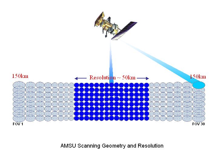
The Advanced Microwave Sounding Unit (AMSU-A), a 15-channel microwave sounder designed primarily to obtain temperature profiles in the upper atmosphere (especially the stratosphere) and to provide a cloud-filtering capability for tropospheric temperature observations. The first AMSU was launched in May 1998 on board the National Oceanic and Atmospheric Administration's (NOAA's) NOAA 15 satellite. The EOS AMSU-A is part of a closely coupled triplet of instruments that include the AIRS and HSB.

Instrument characteristics
*) Passive multi-channel microwave radiometer measuring atmospheric temperature.
*) 15 channel microwave sounder with a frequency range of 15-90 GHz.
*) Provides atmospheric temperature measurements from the surface up to 40 km.
*) On board NOAA K/L/M as well as Aqua.

Moustafa Chahine
AIRS/AMSU/HSB Science Team Leader


Humidity Sounder for Brazil (HSB)

The Humidity Sounder for Brazil (HSB), a 4-channel microwave sounder provided by Brazil aimed at obtaining humidity profiles throughout the atmosphere. The HSB is the instrument in the AIRS/AMSU-A/HSB triplet that allows humidity measurements even under conditions of heavy cloudiness and haze. The HSB provided high quality data until February 2003.

Moustafa Chahine
AIRS/AMSU/HSB Science Team Leader


Advanced Microwave Scanning Radiometer for EOS (AMSR-E)

The Advanced Microwave Scanning Radiometer for EOS (AMSR-E) is a twelve-channel, six-frequency, total power passive-microwave radiometer system. It measures brightness temperatures at 6.925, 10.65, 18.7, 23.8, 36.5, and 89.0 GHz. Vertically and horizontally polarized measurements are taken at all channels. The Earth-emitted microwave radiation is collected by an offset parabolic reflector 1.6 meters in diameter that scans across the Earth along an imaginary conical surface, maintaining a constant Earth incidence angle of 55° and providing a swath width array of six feedhorns which then carry the radiation to radiometers for measurement. Calibration is accomplished with observations of cosmic background radiation and an on-board warm target. Spatial resolution of the individual measurements varies from 5.4 km at 89.0 GHz to 56 km at 6.9 GHz.

Instrument characteristics
*) Passive microwave radiometer, twelve channels, six frequencies, dual polarization, conically scanning.
*) Measures precipitation rate, cloud water, water vapor, sea surface winds, sea surface temperature, ice, snow, and soil moisture.
*) All-weather measurements of geophysical parameters supporting several global change science and monitoring efforts.
*) External cold load reflector and a warm load for calibration.
*) Offset parabolic reflector, 1.6 m in diameter, and rotating drum at 40 rpm.
*) Multiple feedhorns (6) to cover six bands from 6.9 to 89 GHz with 0.3 to 1.1 K radiometric sensitivity; vertical and horizontal polarization.

Roy Spencer
U.S. AMSR-E Science Team Leader


Dr. Spencer received his B.S. in Atmospheric Sciences from the University of Michigan in 1978 and his M.S. and Ph.D. in Meteorology from the University of Wisconsin in 1980 and 1982. He then continued at the University of Wisconsin through 1984 in the Space Science and Engineering Center as a research scientist. He joined NASA's Marshall Space Flight Center (MSFC) in 1984, where he later became Senior Scientist for Climate Studies. He resigned from NASA in 2001 and joined the Univeristy of Alabama in Huntsville as a Principal Research Scientist. Dr. Spencer has served as Pricipal Investigator on the Global Precipitation Studies with Nimbus-7 and DMSP SSM/I, and the Advanced Microwave Precipitation Radiometer High Altitude Studies of Precipitation Systems. He has been a member of several science teams: the Tropical Rainfall Measuring Mission (TRMM) Space Station Accommodations Analysis Study Team, Science Steering Group for TRMM, TOVS Pathfinder Working Group, NASA Headquarters Earth Science and Applications Advisory Subcommittee, and two National Research Council study panels.

Since 1992 Dr. Spencer has been the U.S. Team Leader for the Multichannel Imaging Microwave Radiometer (MIMR) team and the follow-on AMSR-E team. In 1994 he became the AMSR-E Science Team leader.

He received the NASA Exceptional Scientific Achievement Medal in 1991, the MSFC Center Director’s Commendation in 1989, and the American Meteorological Society’s Special Award in 1996.

Selected Papers
Satellite and Model Evidence Against Substantial Manmade Climate Change
Global Warming as a Natural Response to Cloud Changes Associated with the Pacific Decadal Oscillation (PDO)
Cloud and Radiation Budget Changes Associated with Tropical Intraseasonal Oscillations
Potential Biases in Feedback Diagnosis from Observational Data: A Simple Model Demonstration

Akira Shibata
Japanese AMSR-E Science Team Leader

Dr. Akira Shibata, co-leader of the Joint AMSR Science Team, received his B.S., M.S. and Ph.D. from Waseda University, in the Science and Engineering Department. Before moving to the Meteorological Research Institute (MRI) in 1983, he was a technical officer at the Nagasaki Marine Observatory. At MRI he worked as a research scientist. In 1996, Dr, Shibata moved to the Earth Observation Research Center as an Associate senior scientist. He also serves as the ADEOS II AMSR Science Team Leader

Moderate Resolution Imaging Spectroradiometer (MODIS)

The Moderate Resolution Imaging Spectroradiometer (MODIS), is a 36-band spectroradiometer measuring visible and infrared radiation and obtaining data that are being used to derive products ranging from vegetation, land surface cover, and ocean chlorophyll fluorescence to cloud and aerosol properties, fire occurrence, snow cover on the land, and sea ice cover on the oceans. The first MODIS instrument was launched on board the Terra satellite in December 1999, and the second was launched on Aqua in May 2002.

Instrument characteristics
*) Selected for flight on Terra (launched Dec. 1999) and Aqua.
*) Medium-resolution, multi-spectral, cross-track scanning radiometer.
*) Measures physical properties of the atmosphere, and biological and physical properties of the oceans and land.
*) 36 spectral bands—21 within 0.4-3.0 µm; 15 within 3-14.5 µm.
*) Continuous global coverage every 1 to 2 days.
*) Signal-to-noise ratios from 900 to 1300 for 1 km ocean color bands at 70° solar zenith angle.
*) NEDT's typically < 0.05 K at 300K.
8) Absolute irradiance accuracy of 5% for <3 µm and 1% for >3 µm.
*) Daylight reflection and day/night emission spectral imaging.

Michael King
MODIS Team Leader


Dr. Michael King is Senior Research Associate in the Laboratory for Atmospheric and Space Physics, University of Colorado. He served as Senior Project Scientist of NASA's Earth Observing System (EOS) from 1992 to 2008. He joined Goddard Space Flight Center in January 1978 as a physical scientist, and previously served as Project Scientist of the Earth Radiation Budget Experiment (ERBE) from 1983-1992.

His research experience includes conceiving, developing, and operating multispectral scanning radiometers from a number of aircraft platforms in field experiments ranging from arctic stratus clouds to smoke from the Kuwait oil fires and biomass burning in Brazil and southern Africa. He has lectured on global change on all seven continents.

Earlier, he developed the Cloud Absorption Radiometer for studying the absorption properties of optically thick clouds as well as the bidirectional reflectance properties of many natural surfaces, and is principal investigator of the MODIS Airborne Simulator, an imaging spectrometer that flies onboard the NASA ER-2 aircraft. This instrument has aided immeasurably in the development of atmospheric and land remote sensing algorithms for the Moderate Resolution Imaging Spectroradiometer (MODIS) instrument.

Selected Papers
Evaluation of cirrus cloud properties derived from MODIS data using cloud properties derived from ground-based observations collected at the ARM SGP site.
Urban aerosols and their interaction with clouds and rainfall: A case study for New York and Houston.
Observed Land Impacts on Clouds, Water Vapor, and Rainfall at Continental Scales.
Remote sensing of liquid water and ice cloud optical thickness, and effective radius in the arctic: Application of airborne multispectral MAS data.

Cloud's and the Earth's Radiant Energy System (CERES)

The Cloud's and the Earth's Radiant Energy System (CERES) is a 3-channel radiometer measuring reflected solar radiation in the 0.3-5 µm wavelength band, emitted terrestrial radiation in the 8-12 µm band, and total radiation from 0.3 µm to beyond 100 µm. These data are being used to measure the Earth's total thermal radiation budget, and, in combination with MODIS data, detailed information about clouds. The first CERES instrument was launched on the Tropical Rainfall Measuring Mission (TRMM) satellite in November 1997; the second and third CERES instuments were launched on the Terra satellite in December 1999; and the fourth and fifth CERES instruments are on board the Aqua satellite.

Instrument characteristics
*) Selected for flight on TRMM, Terra, and Aqua.
*) Two broadband, scanning radiometers: One cross-track mode, one rotating azimuth plane (bi-axial scanning).
*) First instrument (cross-track scanning) is continuing ERBE, TRMM, and Terra measurements and the second (biaxially scanning) is providing angular radiance information to improve the accuracy of angular models used to derive the Earth's radiative balance.
*) Single scanner on TRMM mission (launched Nov. 1997)
*) Dual scanners on Terra (launched Dec. 1999) and Aqua, and single thereafter.

Bruce Wielicki
CERES Science Team Leader

Dr. Wielicki's research has focused on clouds and their role in the Earth's radiative energy balance for over 20 years. He currently serves as Principal-Investigator on the CERES Investigation and as a Co-Investigator on the NASA Cloudsat and Cloud-Aerosol Lidar and Infrared Pathfinder Satellite Observations (CALIPSO) missions. Cloudsat and CALIPSO are centered on cloud studies and will fly in formation with the CERES instrument and other instruments on the Aqua platform.

Earlier, Dr. Wielicki was a Co-investigator on the Earth Radiation Budget Experiment and developed a new Maximum Likelihood Estimation (MLE) method for determination of the cloud condition in each ERBE field of view. This method enabled the development of the first estimates of cloud radiative forcing (CRF) by distinguishing individual observations as clear, partly-cloudy, mostly-cloudy, or overcast. This measurement became a standard of comparison for global climate models. The poor ability of global climate models to reproduce the ERBE cloud radiative forcing measurements was a key element in the designation of the "role of clouds and radiation" as the highest priority of the U.S. Global Change Research Program.

Dr. Wielicki was also a Principal Investigator on the First International Satellite Cloud Climatology Experiment (ISCCP) Regional Experiment (FIRE) and served as FIRE Project Scientist from 1987 to 1994. His research used Landsat satellite data to provide the first definitive validation of the accuracy of satellite derived cloud fractional coverage. More recently, he has demonstrated the surprising non-gaussian distributions of cloud optical depth present in broken boundary layer cloud fields, and has shown the large bias these distributions can cause in global climate model estimates of both solar and thermal infrared fluxes.

Throughout his career, Dr. Wielicki has pursued extensive theoretical radiative transfer studies of the effects of non-planar cloud geometry on the calculation of radiative fluxes, as well as on the retrieval of cloud properties and top of atmosphere radiative fluxes from space-based observations. Dr. Wielicki received his B.S. degree in Applied Math and Engineering Physics from the University of Wisconsin - Madison in 1974 and his Ph.D. degree in Physical Oceanography from Scripps Institution of Oceanography in 1980. He received a NASA Exceptional Scientific Achievement Award in 1992 and the Henry G. Houghton Award from the American Meteorological Society in 1995.

Selected Papers
Earth's Climate System: A 21st Century Grand Challenge
Ceres And The S'cool Project (1997)
Clouds and the Earth's Radiant Energy System (CERES): An Earth Observing System Experiment
Clouds and the Earth's Radiant Energy System (CERES): algorithm overview

References:
NASA AIRS Web Page
NASA Web Page For Dr. Moustafa Chahine
Retrieval of mid-tropospheric of CO₂ directly from AIRS measurements (2009)
Application of Atmospheric Infrared Sounder (AIRS) data to climate research (2009)
Biases in total precipitable water vapor climatologies from Atmospheric Infrared Sounder and Advanced Microwave Scanning Radiometer (2007)
Three years of hyspersecptral data from AIRS : what have we learned. (2007)
NASA AAMSU-A Web Page
NASA HSB Web Page
NASA AMSR-E Web Page
NASA Web Page For Dr. Roy Spencer
Dr. Spencer's Research Articles Web Page
NASA MODIS Web Page
NASA Web Page For Dr. Michael King
Evaluation of cirrus cloud properties derived from MODIS data using cloud properties derived from ground-based observations collected at the ARM SGP site.
Urban aerosols and their interaction with clouds and rainfall: A case study for New York and Houston.
Observed Land Impacts on Clouds, Water Vapor, and Rainfall at Continental Scales.
Remote sensing of liquid water and ice cloud optical thickness, and effective radius in the arctic: Application of airborne multispectral MAS data.
NASA CERES Web Page
NASA Web Page For Dr. Bruce Wielicki
Earth's Climate System: A 21st Century Grand Challenge
Ceres And The S'cool Project (1997)
Clouds and the Earth's Radiant Energy System (CERES): An Earth Observing System Experiment
Clouds and the Earth's Radiant Energy System (CERES): algorithm overview